
01 · DesignThe parametric model is the dataset specification
Instances, records and files
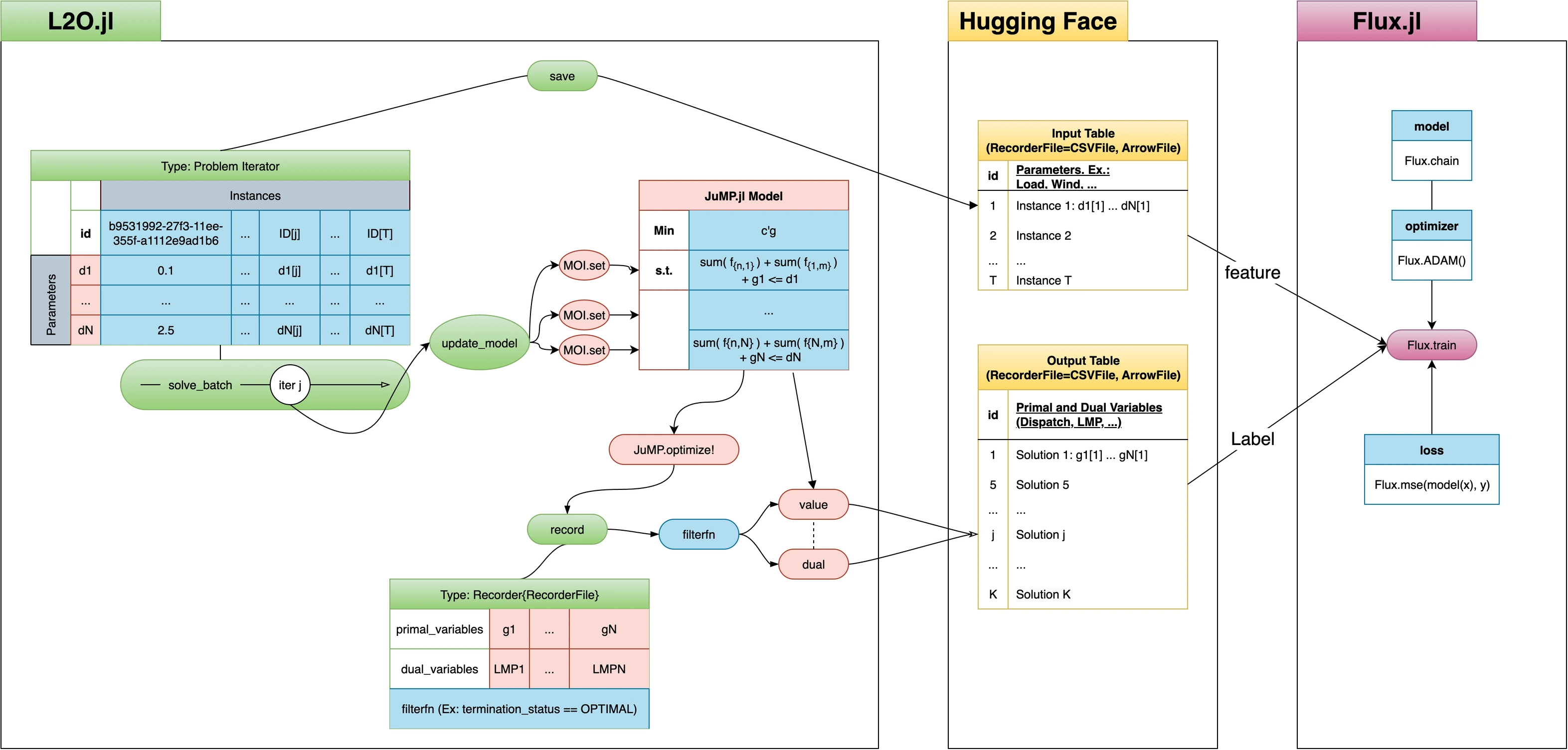
A dataset is specified by a JuMP model whose data are declared as parameters, a ProblemIterator that assigns sampled values to them, and a Recorder that lists the decisions to store and the constraints whose multipliers to store. Samplers draw the values in boxes around the nominal point, along one coordinate at a time, or from scaled distributions, and general_sampler combines them for a model read from a MathOptFormat file. The function solve_batch solves every instance and writes CSV or Arrow tables keyed by a unique identifier per instance, with termination status, objective and solve time; a filter keeps by default only solves with an accepted termination status and feasible primal and dual points.
A dataset is thereby reproducible from a model file and a parameter table, labels can come from any solver that JuMP supports, and the tables match the datasets the organization publishes on Hugging Face.
Sensitivities as labels
When the iterator carries a cotangent \(v_i\) on the decisions of instance \(i\), random by default through random_pullback_primal_pairs, each solve is followed by a DiffOpt.jl reverse pass, and the recorder also stores the vector–Jacobian product \(v_i^\top D_p\mathbf y^\star(p_i)\). The function sobolev_pb_loss_generator builds the corresponding loss for a proxy \(\hat g_\theta\),
with the proxy's product computed by one reverse pass of automatic differentiation.
Derivative supervision then costs one reverse solve per instance and never forms a Jacobian, on either side. This is the unmasked form of the supervision developed on Learning Solution Maps, where a mask selects which sensitivities are matched.
Evaluation in the model's own terms
The evaluators feasibility_evaluator, objective_evaluator and general_evaluator score predicted points against the JuMP model itself: the distance of each constraint function to its set, the objective value, and inference time. The function inconvexhull solves a linear program per query to decide whether a test parameter lies in the convex hull of the training parameters.
A proxy's quality is its constraint violation and objective gap in the original model, and the hull test separates interpolation from extrapolation, which matters for every guarantee that holds only between samples.
Convex and embeddable networks
Networks of type FullyConnected carry the input to every layer through skip connections, and the training rule ConvexRule keeps the weights of every layer after the first nonnegative after each epoch, which makes a scalar output convex in the input. A trained rectified-linear network can be written back into a JuMP model with one binary variable per unit.
A convex network can serve as a convex term of a decision problem, as continuation values do on Continuation-Value Representations; an unrestricted one can be embedded exactly, at the price of integer variables.
The organization
The LearningToOptimize organization hosts, with collaborators, the packages that build on these datasets and models:
- LearningToOptimize.jl: datasets from parametric JuMP models, proxy training and evaluation;
- L2OALM.jl, L2ODLL.jl and L2ODC3.jl: primal–dual learning by the augmented Lagrangian, dual learning, and DC3;
- BatchNLPKernels.jl and BatchConeKernels.jl: GPU kernels that evaluate objectives and constraint violations for batches of nonlinear and conic problems;
- DecisionRules.jl and DecisionRulesExa.jl: policies for multistage problems trained through their stage problems;
- Hugging Face datasets: parametric problems and sensitivity systems.
02 · ExampleA dataset with sensitivity labels
The example follows the package README and its test suite: a one-parameter linear program, ten instances, decisions and multipliers recorded together with one vector–Jacobian product per instance, and the Sobolev loss for a proxy with one input and one output.
using JuMP, Ipopt, LearningToOptimize
import DiffOpt

# A parametric model whose solutions can be differentiated
model = Model(() -> DiffOpt.diff_optimizer(Ipopt.Optimizer))
@variable(model, x)
@variable(model, p in MOI.Parameter(1.0))
@constraint(model, cons, x + p >= 3)
@objective(model, Min, 2x)

# Instances, with one random cotangent on the decisions per instance
problem_iterator = ProblemIterator(Dict(p => collect(1.0:10.0)))
problem_iterator.pullback_primal_pairs = random_pullback_primal_pairs(problem_iterator, 10)
save(problem_iterator, "input", ArrowFile)

# Solve every instance; record decisions, multipliers and vector–Jacobian products
recorder = Recorder{ArrowFile}("output"; primal_variables = [x], dual_variables = [cons])
solve_batch(problem_iterator, recorder)

# Loss on values and pullbacks for a proxy with one input and one output
loss = sobolev_pb_loss_generator(500, 1, 1)
Replacing the model by a PowerModels optimal power flow with nodal demands as parameters, and the iterator by general_sampler on its MathOptFormat file, gives the datasets of the repository's PGLib examples.
03 · ResearchWhere the package carries the theory
- Learning Solution Maps. The supervision developed there, decisions together with selected sensitivities of the solution map, is the kind of dataset this package records, and its Sobolev loss is the unmasked case; the organization also hosts an implementation of the primal–dual construction described there.
- Continuation-Value Representations. The repository's PGLib examples generate operating-value datasets over sampled demand, train input-convex networks with the nonnegativity rule, and test whether a query lies in the hull of the training inputs, the three steps of the study on that page.
04 · CitationHow to cite
For sensitivity-supervised proxies:
@inproceedings{rosemberg2026masked,
  title     = {Masked Sobolev Training for Feasibility-Reliable Optimization Proxies},
  author    = {Rosemberg, Andrew W. and Dias Garcia, Joaquim and Bent, Russell and Van Hentenryck, Pascal},
  booktitle = {Advances in Neural Information Processing Systems},
  year      = {2026}
}
For input-convex value functions:
@article{rosemberg2024learning,
  title   = {Learning Optimal Power Flow Value Functions with Input-Convex Neural Networks},
  author  = {Rosemberg, Andrew and Tanneau, Mathieu and Fanzeres, Bruno and Garcia, Joaquim and Van Hentenryck, Pascal},
  journal = {Electric Power Systems Research},
  volume  = {235},
  pages   = {110643},
  year    = {2024},
  doi     = {10.1016/j.epsr.2024.110643}
}
For the package itself:
@misc{rosemberg_learningtooptimize,
  author       = {Rosemberg, Andrew W.},
  title        = {{LearningToOptimize.jl}: Datasets and proxies for parametric optimization},
  howpublished = {\url{https://github.com/LearningToOptimize/LearningToOptimize.jl}},
  note         = {Julia package}
}