

01 · Selected mapsRepeated solution defines the object to be approximated
Repeated optimization problems define a map from changing problem data to the decisions returned by a specified solution procedure. Let \(p\in\mathcal P\subset\mathbb R^d\) denote the data of a constrained problem with decisions \(\mathbf y\in\mathbb R^n\), objective \(f\), equality system \(c\), and inequality system \(h\). A specified solution procedure returns a selected decision
When the problem has several solutions, \(g\) denotes the solution the procedure returns, and the sensitivities supervised below are those of this selected map, so the choice of solution fixes the training target. Across related instances, \(p\mapsto g(p)\) is the repeated computation, and amortized optimization replaces it by a learned map \(\hat g_\theta\) evaluated in one forward pass (Amos, 2023; Van Hentenryck, 2025; Kotary et al., 2021).
The difficulty lies in the geometry of \(g\). A constrained solution map is smooth only within regions where the active set is stable. As the active set changes, the parameter space splits into critical regions whose number can grow combinatorially with the number of constraints, so generalization from finitely many samples and constraint behavior between them are the central questions of any construction.
Direct solution matching uses solved pairs \(\{(p_i,g(p_i))\}_{i=1}^N\) and empirical risk minimization,
Here \(\theta\) denotes the proxy weights and \(\ell\) the decision loss, giving the standard construction of optimization proxies (Pan et al., 2020; Chatzos et al., 2020). In imitation learning, the same objective defines behavior cloning, with the solver as the expert. It retains only the relation between an instance and a returned decision. The feasibility mechanism, the optimality system, and the selection that produced each label are absent, so low average decision error can coexist with poor interpolation between sampled regions, constraint violations, and heavy tails. Out of distribution these errors grow, because a new parameter may require an active set that none of the training pairs exhibits, even within the range the data cover. The construction also presumes that a selected solution can be computed offline for every training instance.

02 · Retained structureThe constrained problem, or its solver, can remain in the construction
When selected labels are unavailable, incomplete, or too costly at scale, the optimization model can supply the training signal itself. Self-supervised primal–dual learning (Park and Van Hentenryck, 2023) follows an augmented-Lagrangian method with two maps: a primal map \(\hat{\mathbf y}=\hat g_\theta(p)\) and an instance-conditioned dual map \((\hat{\boldsymbol\lambda},\hat{\boldsymbol\mu})=\Lambda_\psi(p)\) for the multipliers of \(c\) and \(h\). With the dual map frozen, the primal map minimizes
Here \(\psi\) denotes the dual map's weights, \(\hat{\mathbf y}_i=\hat g_\theta(p_i)\), the hatted multipliers are the dual map's outputs at \(p_i\), \(\rho>0\) is the penalty coefficient, \([\,\cdot\,]_+\) is the componentwise positive part, and \(f_i,c_i,h_i\) abbreviate the corresponding evaluations at \((\hat{\mathbf y}_i,p_i)\).
With the primal map frozen, the dual map is regressed onto the multiplier step of the method:
Here \((\boldsymbol\lambda_k,\boldsymbol\mu_k)\) come from a copy of the dual map taken at the start of outer iteration \(k\), and \(\rho\) grows when the largest violation stops decreasing. The second network is there to hold instance-specific multipliers, which an augmented-Lagrangian method would otherwise store and update for every training instance, and which earlier Lagrangian-dual training shared across instances (Fioretto et al., 2020).

The criterion is self-supervised: The signal comes from the objective and the constraint residuals, without precomputed solutions. Neither this criterion nor regression makes a raw prediction feasible. When a repair, completion, or projection map is inexpensive and differentiable, or directionally differentiable, it can be composed with the proxy to recover feasible outputs (Donti et al., 2021; Qiu et al., 2024), and the completed decision becomes the object to evaluate.
Learned coefficients of a retained model
A third construction keeps the solver as the decision engine. A map conditioned on the context \(w\) selects the coefficients \(p\) of a tractable model, and the model computes the decision:
The learned object is a coefficient map, judged by the induced decision against a detailed model rather than by coefficient error. This is the right allocation when a tractable model carries structure worth retaining, such as an explicit feasible region, operational logic, or an interface to another computation, while its fixed coefficients are inadequate across contexts. Learned Model Correction develops it (Rosemberg et al., 2025b).
The three constructions differ in what they keep at deployment: a direct proxy, a completed prediction, or a solve with learned coefficients. A separate requirement appears when the learned map is itself placed inside a computation that is differentiated.
03 · Local fidelityA decision-accurate proxy can transmit the wrong local response
Let \(L\) be any computation that uses the map: a downstream optimization, a controller, or the objective of a policy being trained. Its gradient passes through the Jacobian of the map,
Here \(Dg\) is the Jacobian of the selected map; a proxy fitted to decisions leaves \(D\hat g_\theta\) unsupervised. It can predict decisions accurately and still return the wrong gradient to every computation built on it, so for a proxy that replaces a solve inside a differentiated pipeline the local response is part of the object being approximated.
At a regular selected solution that response is computable. Collect the primal–dual solution in \(\mathbf z^\star(p)\) and the stationarity, feasibility, and complementarity conditions in \(F(\mathbf z,p)=\mathbf 0\). Under the linear independence constraint qualification, a second-order sufficient condition, and strict complementarity (Fiacco, 1976), the implicit function theorem gives
Here \(F_{\mathbf z}\) and \(F_p\) denote the two partial Jacobians evaluated at the selected solution, so the sensitivity is obtained by a linear solve with the KKT matrix. The primal block of \(D_p\mathbf z^\star\) is \(Dg(p)\), a solution sensitivity. The derivative of the optimal value follows from the multipliers by the envelope theorem, and it suffices only when \(L\) depends on the inner problem through that value. The construction, its failure modes, and its implementation in existing modeling languages are treated in Differentiating Optimization Models (Rosemberg et al., 2025a).
Masked Sobolev training (Rosemberg et al., 2026a) supervises both objects. Sobolev training matches derivatives as well as values (Czarnecki et al., 2017), derivative supervision has been used for surrogates embedded in optimization models (Tsay, 2021), and derivative matching, explicit or through implicit regularization, has reduced generalization error on optimization-related prediction (Zhang et al., 2022; Rosemberg et al., 2024); here the derivative labels are the sensitivities of a solver-selected constrained map. For each sampled \(p_i\), the solver supplies \(g(p_i)\) and a differentiable-optimization layer supplies \(Dg(p_i)\); during training, automatic differentiation supplies \(D\hat g_\theta(p_i)\), and a binary mask \(M\in\{0,1\}^{n\times d}\) selects the Jacobian entries that enter an update:
Here \(\ell_d\) measures sensitivity discrepancy, \(\gamma\ge0\) weights derivative supervision, and \(\odot\) denotes entrywise multiplication.

At each update a fresh mask selects \(K\) of the \(nd\) entries uniformly, so each entry is included with probability \(K/(nd)\). Write \(A=D\hat g_\theta(p_i)-Dg(p_i)\) and, for \(K\in\{1,\ldots,nd\}\), normalize the derivative loss by the number of retained entries:
Here \(\mathcal M_K\) is the set of masks with exactly \(K\) retained entries, \(\operatorname{Unif}\) is its uniform law, \(\lVert\,\cdot\,\rVert_F\) is the Frobenius norm, and \(\lVert M\rVert_0\) counts the retained entries; the expectation holds \(p_i\) and \(\theta\) fixed and establishes unbiasedness for dense Jacobian matching. The weight \(\gamma\) sets the strength of derivative supervision; the mask density sets how many Jacobian conditions act on the network in the same update. Density matters on its own because sensitivities computed in different active-set regimes impose competing conditions on one network, a contention akin to gradient conflict in constrained learning (Liu et al., 2024). A sparse mask that changes at every update lets those conditions enter gradually. The mask is uniform by design; it controls only how many entries are matched at once.

The derivative term composes with the constructions of Section 02. It can be added to a self-supervised objective, and it can shape the response of a proxy whose last layer is a differentiable repair or completion, before or through that layer. In every case the solver, the sensitivity computation, and the proxy Jacobian are used only in training; inference remains one forward pass.
Where first-order labels are valid
An approximation statement identifies the regime in which a derivative at a sample describes its neighborhood. Let \(\mathcal P\) be compact and convex, and let the samples have covering radius \(\delta=\sup_{p\in\mathcal P}\min_i\lVert p-p_i\rVert\). Assume exact interpolation at the samples, an idealization that the training objective does not guarantee. If \(g\) and \(\hat g_\theta\) are Lipschitz with constants \(K_g,K_{\hat g}\), value interpolation gives the first bound below. If both are continuously differentiable with Jacobians Lipschitz with constants \(K'_g,K'_{\hat g}\) (\(L_g\) and \(M_g\) in the paper), joint value-and-Jacobian interpolation removes the constant and first-order error at every sample, and the error between samples becomes second order (Rosemberg et al., 2026a, Theorems 1 and 3):
The regularity conditions above give local differentiability of a suitably selected map, and networks with smooth activations of bounded curvature satisfy the proxy's conditions on compact sets. The Jacobian-Lipschitz condition requires more: The sensitivities must vary slowly over the region considered. The bounds therefore hold region by region where both maps are regular. They are not a convergence result for masked training, and they make no claim across arbitrary active-set transitions. A transition does not by itself make a derivative label useless. A sensitivity that has ceased to be the exact local derivative still helps when neighboring sensitivities are similar, while a sharp change of the Jacobian limits what matching can add. Discrete decisions, disjunctions, and other nonsmooth structure lie outside this setting and require surrogate sensitivities from relaxations, smoothing, or duality.
04 · Problem classesThe geometry of the selected map decides what derivative labels add
Three studies hold the comparison fixed and change the geometry of the selected map. In each, a value-only proxy and a masked Sobolev proxy share the architecture and the training pipeline, so the differences come from the derivative labels. Each study is paired with a computed two-parameter instance of the same problem class, which shows the geometry the proxy has to interpolate.
A smooth map: distilling a feedback controller
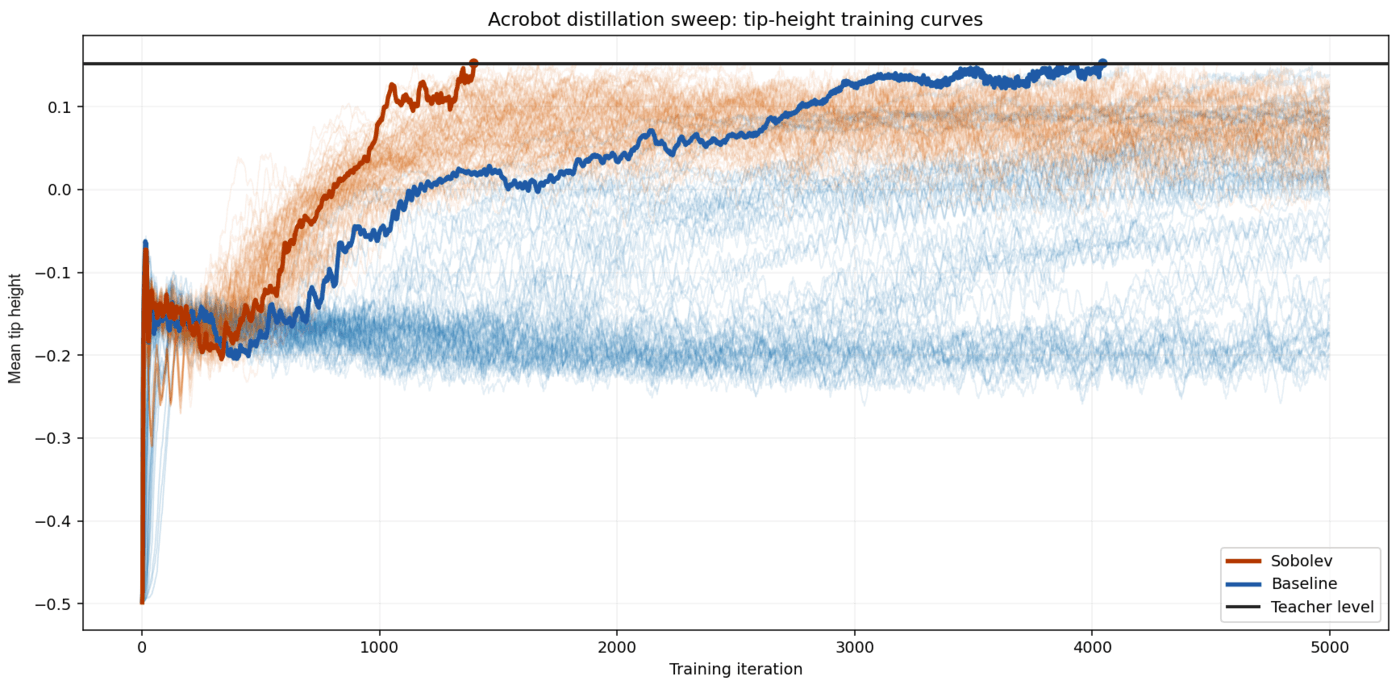
The first study is finite-horizon optimal control of an underactuated two-link pendulum, the Acrobot swing-up. The parameter is the initial state \(p=\mathbf x_0\), and the map returns the first action of the optimal trajectory, which makes it a feedback policy. Apart from an actuator box the constraints are the smooth dynamics, so the map rarely changes active set. The reference map is a feedback controller trained on the same objective by proximal policy optimization (Schulman et al., 2017), and its action sensitivities with respect to the state, computed by automatic differentiation, are the derivative labels. A trained teacher makes the study an instance of policy distillation and separates the effect of first-order supervision from solver-specific multiplier and factorization conventions. Both students are trained with DAgger relabeling, and each method receives 192 runs over its hyperparameter sweep.
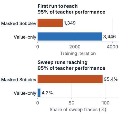
Both highlighted runs eventually reach the teacher's level, so the labels change how quickly and how reliably learning proceeds. At a common threshold of 95% of teacher performance, the first Sobolev run crosses at iteration 1,349 and the first value-only run at iteration 3,446, about 2.5 times fewer iterations; despite a 2% higher cost per iteration, that is about 16 minutes against 40. Across the sweeps, 95.4% of Sobolev runs reach the threshold, against 4.2% of value-only runs.

Many active-set regimes: AC optimal power flow
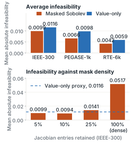
AC optimal power flow keeps the object, a parametric solution map, and removes the simplifying structure. Demand is the parameter; the decisions collect generation, voltages, and branch flows; \(c\) holds the nonlinear power-flow equations and \(h\) the operating limits. The limits partition the demand space into active-set regimes whose number can grow combinatorially. Within a regime, KKT sensitivities describe how decisions move along the binding constraints; by themselves they do not describe the neighboring regimes, and a proxy with small decision error can still violate operating limits. Reliability is therefore judged by objective gap and constraint violation. The proxies have two hidden layers of width 320 and are trained on about 10,000 instances of three networks from the PGLib benchmark library (Babaeinejadsarookolaee et al., 2019) with up to 6,468 buses, retaining 5% of Jacobian entries on IEEE-300 and PEGASE-1k and 25% on RTE-6k.
Masked Sobolev training lowers average infeasibility on all three networks, and the tails carry the stronger result. Instance by instance, the Sobolev proxy has the larger worst-case violation on fewer than 15% of test instances, and the median improvement in worst-case violation, normalized by the largest Sobolev violation on each test set, is about 18%, 400%, and 180% on the three networks. Objective gaps stay at or below 0.22%; the value-only proxy has the smaller gap on IEEE-300 and PEGASE-1k (0.02% against 0.22%, and 0.07% against 0.15%), and the two coincide at 0.07% on RTE-6k. No repair layer is used; the remaining violations are mostly small power-flow mismatches.
The gain depends on the mask. On IEEE-300, retaining 5–10% of the Jacobian entries gives the lowest infeasibility; beyond 25% infeasibility rises sharply, and dense matching has more than five times the infeasibility of the 5% mask and exceeds the value-only proxy. Because the normalization keeps the expected derivative loss fixed, the comparison changes how many conditions act at once without changing the expected weight of the derivative term. The labels add training cost and leave inference unchanged: On RTE-6k an epoch takes about 1.6 times as long.

Sparse solutions: mean–variance allocation
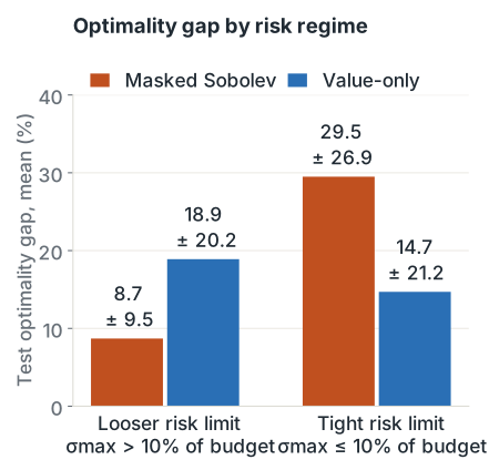
The third study keeps the problem convex and the sensitivities locally valid, but makes them nearly uninformative. Mean–variance selection over 500 assets maximizes expected return under a second-order-cone risk limit \(\sigma_{\max}\) and a budget. In the data, fewer than 15% of assets typically receive more than 0.01% of the budget, so most sensitivities are zero or very small, and small changes of the returns or of the risk limit change which assets are active. Regression on reference portfolios gave mean gaps above 90%, so both proxies train on the portfolio objective through a feasibility-preserving output layer, the composed construction of Section 02, and the Sobolev proxy adds solver sensitivities as derivative labels.
Outside the tightest risk limits, derivative labels more than halve the test gap: 8.7 ± 9.5% against 18.9 ± 20.2%. Under tight limits, \(\sigma_{\max}\le 10\%\) of the budget, where allocations are sparsest, they worsen it: 29.5 ± 26.9% against 14.7 ± 21.2%. The split points to using derivative supervision only where it is informative, for example through regime-specific models; the study does not test that remedy.

Across the three classes, a derivative label is worth what the sensitivity at its sample says about the neighborhood. Where it describes the region the proxy must learn, the labels accelerate learning and improve constraint satisfaction, provided the mask keeps the conditions of different regimes from competing. Where it does not, they add little and can degrade the proxy. The same reading applies to multipliers and solution sensitivities used anywhere as a learning signal: The local response of an optimization model teaches to the extent that it describes the neighborhood of the point at which it is computed.
05 · Sequential useA policy can supply the reference map or use the learned one
One student from several teachers
Many systems are operated by specialized controllers, each competent on part of the task and obtained by optimization, expert design, or policy-gradient training. The construction then distills a family of reference maps into one student that meets the observation and latency requirements of deployment. One application explored in this research is in-hand reorientation by a multi-fingered robot, which rotates grasped objects of different geometries about a target yaw direction while keeping a stable grasp. Even object-specific teachers are hard to construct, so supervision is uneven in quality across objects, and reusable supervision for high-dimensional dexterous control is itself a current concern (de Bakker et al., 2025).
Let \(\pi^{\mathrm{tch}}_b\) be the teacher for object \(b\) and \(\pi^{\mathrm{stu}}(\cdot\,;\theta)\) the shared student. The student observes delayed or noisy proprioception, its previous command, and an encoding of the point cloud from a wrist-mounted sensor, and acts through joint-position increments \(\mathbf y_t\in[-1/24,\,1/24]^{16}\). The object index selects the teacher and the environment but is not an input to the student, and states visited by the student are relabeled by the corresponding teacher. Action matching and its Sobolev variant use
Here \(e_b\) is the action discrepancy, \(\mathcal I\) indexes the objects, \(\nu_\theta(\,\cdot\mid b)\) is the law of student-visited observations on object \(b\), \(\hat o\) selects each teacher's inputs from the common observation coordinates, and random vectors \(v_m\in\mathbb R^{16}\), \(m=1,\ldots,R\), project the action sensitivities, so that \(R\) vector–Jacobian products replace complete Jacobians, as in the stochastic projections of Sobolev training (Czarnecki et al., 2017).
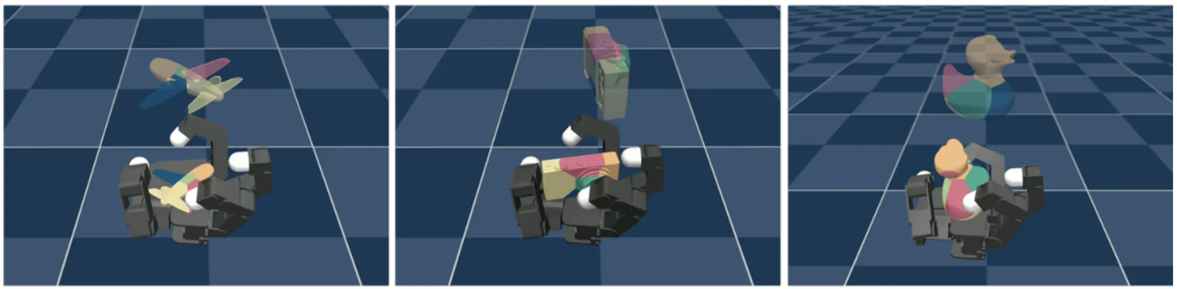
Matching local responses as well as actions is the construction for teachers of uneven quality, and its criterion is held-out task success over repeated seeds at matched student architecture, observations, samples, and training budget. Optimization-based controllers and learned proxies can join the teacher set, and their local responses are exactly the sensitivities of Section 03. One boundary is structural. When a teacher acts on privileged information, two states that the student cannot distinguish can receive different teacher actions, which a memoryless student cannot represent; the study begins from compatible observations to separate the multi-teacher question from that ambiguity. In early exploration, matching local responses already raises the final success on two thirds of the objects. Its effect on learning speed is larger: the shared policy reaches 95% of the level attained by action matching in 23% fewer epochs, and early in training it succeeds up to nearly twice as often. Further work is needed to generalize to unseen objects whose geometry departs far from that of the teacher set.
Recourse inside a policy
For a state-target policy, stage recourse is itself a selected solution map. Its parameters are the incoming state, the prescribed target, and the revealed uncertainty, and \(E\) extracts the applied controls from the returned solution:
Here \(\mathbf y_t^\star\) and \(\hat{\mathbf y}_t\) are the selected and proxy controls, respectively. AC optimal power flow is the kind of nonconvex recourse whose solve time sets the cost of each decision of such a policy. Replacing the solve changes more than execution time. Decision error and constraint violations propagate through the realized transitions, and Jacobian error changes the signal available to the surrounding policy search. A learned solution map does not by itself define a policy; it becomes the recourse component through which a policy is realized and trained. Policies for Multistage Decisions develops that policy.
Software
LearningToOptimize records the solved instances, multipliers, and sensitivity labels that this supervision needs from any parametric JuMP model, and DiffOpt.jl computes the sensitivities at each sampled solution.

LearningToOptimize
Turns a parametric JuMP model into datasets of decisions, multipliers and sensitivities, and trains and evaluates optimization proxies on them.

DiffOpt.jl
Solution and optimal-value derivatives of JuMP models with respect to named parameters, through the model's reformulations, for convex and smooth nonconvex programs.
References
- B. Amos. Tutorial on amortized optimization. Foundations and Trends in Machine Learning 16(5):592–732, 2023.
- S. Babaeinejadsarookolaee, A. Birchfield, R. D. Christie, C. Coffrin, C. DeMarco, R. Diao, M. Ferris, S. Fliscounakis, S. Greene, R. Huang, et al. The power grid library for benchmarking AC optimal power flow algorithms. Preprint arXiv:1908.02788, 2019.
- M. Chatzos, F. Fioretto, T. W. K. Mak, P. Van Hentenryck. High-Fidelity Machine Learning Approximations of Large-Scale Optimal Power Flow. Preprint arXiv:2006.16356, 2020.
- W. M. Czarnecki, S. Osindero, M. Jaderberg, G. Swirszcz, R. Pascanu. Sobolev training for neural networks. Advances in Neural Information Processing Systems 30, 2017.
- V. de Bakker, J. Hejna, T. G. W. Lum, O. Celik, A. Taranovic, D. Blessing, G. Neumann, J. Bohg, D. Sadigh. Scaffolding dexterous manipulation with vision-language models. Preprint arXiv:2506.19212, 2025.
- P. L. Donti, D. Rolnick, J. Z. Kolter. DC3: A learning method for optimization with hard constraints. International Conference on Learning Representations, 2021.
- A. V. Fiacco. Sensitivity analysis for nonlinear programming using penalty methods. Mathematical Programming 10(1):287–311, 1976.
- F. Fioretto, T. W. K. Mak, P. Van Hentenryck. Predicting AC optimal power flows: Combining deep learning and Lagrangian dual methods. Proceedings of the AAAI Conference on Artificial Intelligence 34:630–637, 2020.
- J. Kotary, F. Fioretto, P. Van Hentenryck, B. Wilder. End-to-end constrained optimization learning: A survey. Proceedings of the International Joint Conference on Artificial Intelligence, pp. 4475–4482, 2021.
- Q. Liu, M. Chu, N. Thuerey. ConFIG: Towards conflict-free training of physics informed neural networks. Preprint arXiv:2408.11104, 2024.
- X. Pan, T. Zhao, M. Chen, S. Zhang. DeepOPF: A deep neural network approach for security-constrained DC optimal power flow. IEEE Transactions on Power Systems 36(3):1725–1735, 2020.
- S. Park, P. Van Hentenryck. Self-supervised primal-dual learning for constrained optimization. Proceedings of the AAAI Conference on Artificial Intelligence 37(4):4052–4060, 2023.
- G. Qiu, M. Tanneau, P. Van Hentenryck. Dual conic proxies for AC optimal power flow. Electric Power Systems Research 236:110661, 2024.
- J. Schulman, F. Wolski, P. Dhariwal, A. Radford, O. Klimov. Proximal policy optimization algorithms. Preprint arXiv:1707.06347, 2017.
- C. Tsay. Sobolev trained neural network surrogate models for optimization. Computers & Chemical Engineering 153:107419, 2021.
- P. Van Hentenryck. Optimization learning. Preprint arXiv:2501.03443, 2025.
- L. Zhang, Y. Chen, B. Zhang. A convex neural network solver for DCOPF with generalization guarantees. IEEE Transactions on Control of Network Systems 9(2):719–730, 2022.
- A. Rosemberg, M. Tanneau, B. Fanzeres, J. Garcia, P. Van Hentenryck. Learning optimal power flow value functions with input-convex neural networks. Electric Power Systems Research 235:110643, 2024. DOI 10.1016/j.epsr.2024.110643.
- A. W. Rosemberg, J. Dias Garcia, F. Pacaud, R. B. Parker, B. Legat, K. Sundar, R. Bent, P. Van Hentenryck. A general and streamlined differentiable optimization framework. Preprint arXiv:2510.25986, 2025.
- A. Rosemberg, M. Klamkin, P. Van Hentenryck. Differentiable optimization for deep learning-enhanced DC approximation of AC optimal power flow. NeurIPS 2025 Workshop on Mathematical Foundations and Operational Integration of Machine Learning for Uncertainty-Aware Decision-Making (MLxOR), arXiv:2504.01970, 2025.
- A. W. Rosemberg, J. Dias Garcia, R. Bent, P. Van Hentenryck. Masked Sobolev training for feasibility-reliable optimization proxies. Advances in Neural Information Processing Systems, 2026. Earlier preprint: Sobolev training of end-to-end optimization proxies, arXiv:2505.11342, 2025.
Publication
The paper is presented at NeurIPS 2026 (conference poster page). Its website carries interactive versions of the three computed instances above.
Masked Sobolev Training for Feasibility-Reliable Optimization Proxies
Earlier preprint: Sobolev Training of End-to-End Optimization Proxies (arXiv, 2025).
Paper websiteNeurIPS page arXivBibTeX
@inproceedings{rosemberg2026masked,
  title     = {Masked Sobolev Training for Feasibility-Reliable Optimization Proxies},
  author    = {Rosemberg, Andrew W. and Dias Garcia, Joaquim and Bent, Russell and Van Hentenryck, Pascal},
  booktitle = {Advances in Neural Information Processing Systems},
  year      = {2026}
}