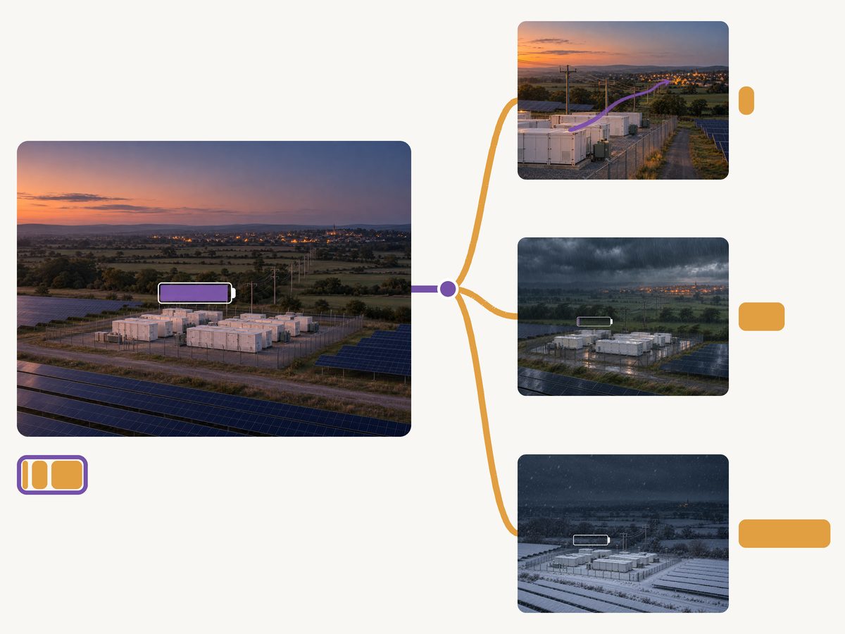
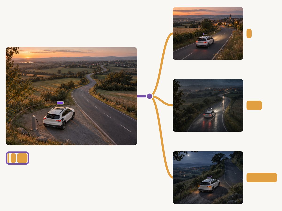
01 · Continuation valueThe state decision queries the remaining cost
A decision's future cost depends on the state it leaves for subsequent decisions. At stage \(t\), the incoming state \(\mathbf x_{t-1}\) and the realization \(w_t\) are observed; the outgoing state \(\mathbf x_t\) and the recourse decisions \(\mathbf y_t\) are then selected. Because the state contains every quantity that couples consecutive stages, the future cost depends on the recourse only through \(\mathbf x_t\), and the Bellman recursion separates into two minimizations:
The stage recourse value \(q_t\) is the least operating cost of a proposed transition; \(f\) is the stage cost, \(\mathcal T=\mathbf0\) encodes the transition, \(h\ge\mathbf0\) gives the operating constraints defining \(\mathcal Y_t\), \(n_x,n_y\) are the state and recourse dimensions, \(w_{[t]}=(w_1,\dots,w_t)\) is the observed history, and \(\mathbb P\) is the uncertainty law. The continuation value \(\mathcal V_{t+1}\), with \(V_{T+1}\equiv0\), is the expected optimal cost of the remaining stages given the outgoing state and the observed history. Exact evaluation is intractable in general: With \(B\) realizations at each uncertain stage there are \(B^{T-1}\) paths, and a grid with \(m\) values per state component has \(m^{n_x}\) points, with \(n_x\) the state dimension.
An approximation of \(\mathcal V_{t+1}\) therefore becomes a term of the stage minimization, and its structure determines what that minimization is. It decides whether the term can be written with linear inequalities over continuous variables, which leaves the stage problem in the class of the operating model, whether it needs integer variables, or whether only local solutions are available.
02 · Cutting planesConvexity makes a cut computed at one state valid at every state
Stochastic dual dynamic programming (Pereira and Pinto, 1991) represents the continuation value under stagewise-independent uncertainty by a maximum of affine functions and solves, at each stage,
Here \(\vartheta\) is the epigraph variable for the maximum of \(K\) cuts, with intercepts \(\alpha_k\) and slopes \(\boldsymbol\beta_k\).
A cut is computed at a visited state \(\mathbf x^k\) by solving the next-stage problems with a copy of the incoming state fixed to \(\mathbf x^k\). With exact downstream values, jointly convex stage problems, affine state-fixing constraints, and strong duality, the multiplier \(\boldsymbol\mu_{t+1}\), signed as the sensitivity to the fixed state, is a subgradient of the next-stage value, and its probability-weighted average \(\boldsymbol\beta_k=\mathbb E_{t+1}[\boldsymbol\mu_{t+1}]\) is a subgradient of the continuation value at \(\mathbf x^k\). Convexity then turns local information into a global statement:
Here \(\partial\) denotes the convex subdifferential. In SDDP's backward pass, these solves use the current downstream cuts, and the resulting affine functions lower-bound the continuation value under the same convexity and duality assumptions. Solves at a sampled state improve the approximation across the state space, and each stage remains a convex program with its operating constraints. Under the standard sampling assumptions together with stagewise-independent uncertainty, the first-stage bound is nondecreasing as cuts accumulate and can be compared with the simulated cost of the policy (Shapiro et al., 2009; Füllner and Rebennack, 2025).
For nonconvex stages, the multipliers of a local optimum need not define a global supporting plane, and exact Lagrangian cuts need nonconvex subproblems solved to global optimality (Zou et al., 2019). Applications therefore take cuts from a convex relaxation or approximation and operate the detailed model with them; Planning and Realization Mismatch shows that neither a tight bound nor a tighter relaxation guarantees the better operated policy (Brigatto et al., 2017; Rosemberg et al., 2022).
The cutting-plane machinery needs a convex function from which to take cuts. It does not require that function to be the value of a convex model of the system, which leaves room for a convex function learned from the detailed model.
03 · RepresentationAn input-convex network carries convexity without a convex model
An input-convex neural network (Amos et al., 2017) is convex in its input by construction. The architecture used here carries the input to every layer through skip connections,
Here \(\mathbf a^{l}\) is the output of layer \(l\) of \(L\), \(W^{l}\) and \(U^{l}\) are weight matrices, \(\mathbf d^{l}\) is a bias vector, and \(p\) collects the supplied problem data. In a stage problem, \(p\) may contain incoming and outgoing states and the realized uncertainty; in the study below it contains nodal demand. The rectified linear unit is convex and nondecreasing, so a nonnegative combination of convex outputs of the previous layer remains convex. The skip weights \(U^{l}\) enter affinely and may take either sign, which permits decreasing slopes. A scalar output layer with the same sign restriction gives a convex piecewise-affine prediction \(\hat q(p)\). Training keeps \(W^{l}\) nonnegative by projected gradient updates.
An unrestricted network is generally nonconvex in its input. Embedded in a decision problem, it is either queried as a gray-box function, which yields local solutions only, or, with rectified linear units, written as a mixed-integer program with a binary variable per unit (Fischetti and Jo, 2018; Anderson et al., 2020). An input-convex network can be retained in two convex forms: the whole network through its matrix products and the epigraphs of its activations, exact without integer variables when the network value is minimized (Liu et al., 2026); or cuts generated at queried states,
Here \(\bar{\mathbf x}\) is the queried state and \(\ell\) is its supporting affine cut, which enters the stage problem exactly as the cuts of Section 02. The subgradient, obtained by automatic differentiation, takes the place of the cut slope \(\boldsymbol\beta_k\). Which form solves faster depends on the application and on the size of the network. To serve as a continuation value, the network must be trained on costs that include every later stage.

What the cuts certify
Each cut is an exact support of the network, so it lies below \(\widehat{\mathcal V}_{t+1}\) at every state, and the maximum of any collection of cuts is a lower approximation of the network that tightens as cuts are added. That is the property the cutting-plane algorithm uses. The cuts carry no guaranteed bound on the cost of the detailed model when that cost is nonconvex: Wherever the detailed cost falls below the fitted function, a cut of the fit can exceed it. Convexity of the representation also does not make the stage problem convex; the retained operating constraints still decide that.

Error between samples
When the reference value is convex, sampled values and multipliers bound the error of a convex approximation between the samples. Consider a convex operating value \(q(p)\) with affine right-hand-side perturbations and a strong dual, for example \(q(p)=\min_{\mathbf y}\{\mathbf c^\top\mathbf y:A\mathbf y\ge p\}\), so that an optimal multiplier is a subgradient of \(q\). Let \(\{(p_i,\boldsymbol\mu_i,z_i)\}_{i=1}^N\) be sampled parameters, optimal multipliers, and values, \(P=\operatorname{conv}\{p_1,\dots,p_N\}\), and \(\Omega(p)=\{\boldsymbol\omega\ge0:\sum_i\omega_i=1,\ \sum_i\omega_ip_i=p\}\). The samples define a lower and an upper envelope,
The network envelopes \(\hat q^-,\hat q^+\) are built the same way from the network values \(\hat z_i=\hat q(p_i)\) and subgradients \(\hat{\boldsymbol\mu}_i\in\partial\hat q(p_i)\). If \(q\) and \(\hat q\) are convex and finite on \(P\), then for every \(p\in P\)
This follows because supporting subgradients place each function above its lower envelope and Jensen's inequality places it below its upper envelope. If, in addition, the network matches the values and shares a supporting subgradient at every sample, \(\hat q(p_i)=z_i=q(p_i)\) and \(\boldsymbol\mu_i\in\partial\hat q(p_i)\cap\partial q(p_i)\), then \(|\hat q(p)-q(p)|\le\max_i\lVert\boldsymbol\mu_i\rVert_*\operatorname{diam}(P)\) on \(P\), with \(\lVert\cdot\rVert_*\) the dual of the norm that defines \(\operatorname{diam}(P)\). The bound is computed from samples alone, tightens on the convex hull of any subset of the samples, and shows how matching the multipliers of the reference model, in addition to its values, controls the error between samples. It extends the guarantee of Zhang et al. (2022) to general input-convex networks (paper Theorems 1 and 2; proposal Theorem 3.1).
The statement has two boundaries. It requires a convex reference: The DC and SOC operating values are convex in demand on their feasible domains, but the AC value is not, so neither envelope is guaranteed to enclose it. It holds only on \(P\): With hundreds of demand coordinates, the hull of the training inputs need not contain most test points. In the IEEE-300 study, 22% of the test instances lay inside it with 400 or 6,500 training instances and 43% with 20,000, and the input-convex and unrestricted networks performed alike, with similar mean errors inside and outside the hull and worst errors up to about twice as large outside it at 20,000 training instances (paper Table 3). Yet many nonconvex problems have values that are convex over regions of their parameter space, or nearly convex overall, which makes such generalization statements useful beyond these boundaries.
04 · Operating-value studyA convex representation matches an unrestricted network on the values of a nonconvex model
The completed study tests whether convexity costs accuracy when the network learns the value of a large constrained operating problem. Each value describes one operating period of an optimal power flow and plays the role of the stage recourse value \(q_t\). Three formulations of increasing fidelity are learned: the DC approximation, a linear program; the SOC relaxation (Jabr, 2006), convex and nonlinear; and the AC model, nonconvex, on which the systems are operated. The input is active and reactive nodal demand; network data, limits, and generation costs are fixed.
The systems are four PGLib-OPF cases (Babaeinejadsarookolaee et al., 2019): IEEE-300, PEGASE-1k, PEGASE-2k, and RTE-6k, with 300, 1,354, 2,869, and 6,468 buses. For each, 50,000 instances scale nominal demand by a uniform system-wide factor and independent bus-level log-normal noise with mean one and standard deviation 5%, over a range chosen to avoid AC infeasibility; infeasible instances are excluded and the remaining instances are split 40%, 30%, and 30% into training, validation, and test sets. The input-convex and unrestricted networks share one architecture and differ only in the sign restriction. Error is \(|\hat z-z^\ast|/|z^\ast|\) against the solver value \(z^\ast\), averaged geometrically.

On the AC values, the two networks tie on IEEE-300 (0.39%), and the input-convex network is lower on the other three systems. Its mean error is also below that of the SOC relaxation's optimal value on all four systems and well below the DC approximation's (2.91% to 7.35%). Across the three formulations, its mean errors stay below 0.5% except on the SOC model of PEGASE-2k, where training did not converge (1.03%). The relaxation keeps an advantage the network lacks: Its value is a valid lower bound on the AC value.
Worst errors are much larger and are not uniformly improved by convexity. On IEEE-300 both networks exceed 14%, about 40 times their mean, and on the other systems the worst errors range from 1.95% to 8.89%. The paper attributes the accuracy on AC values to their approximate convexity: Along segments between extreme points of the sampled demand set on IEEE-300, the AC operating cost is mostly convex in the load, with isolated departures (paper Fig. 4), consistent with the tightness of convex relaxations for many systems (Molzahn and Hiskens, 2019). Training on a tail risk measure of the prediction error, such as its conditional value at risk, instead of its empirical mean may reduce the worst errors.

05 · Convex criticA learned continuation value inside policy training
The windowed construction in Policies for Multistage Decisions trains a state policy over windows of \(H\) stages and closes each window with a critic \(\widehat{\mathcal V}^{\pi}\) of the policy's remaining cost (Konda and Tsitsiklis, 1999); the construction and its trade-off between update cost and critic bias are developed there.
The convex representation of Section 03 is a natural critic. Its targets then come from policy evaluation or temporal-difference updates rather than from single-period operating values, and its subgradients play the role of \(\nabla\mathcal V_{t+1}\). Convexity is required only when the critic is also queried inside a convex decision problem; within policy training it acts as a structural prior on the continuation value. When the continuation value is instead computed on a simplified planning model and used to operate a detailed one, the question becomes the mismatch that substitution creates, treated in Planning and Realization Mismatch.
Software
LearningToOptimize generates operating-value datasets from parametric JuMP models, trains input-convex networks with nonnegative weights, and tests whether a query lies in the hull of the training inputs.

LearningToOptimize
Turns a parametric JuMP model into datasets of decisions, multipliers and sensitivities, and trains and evaluates optimization proxies on them.
References
- B. Amos, L. Xu, J. Z. Kolter. Input convex neural networks. International Conference on Machine Learning, PMLR, pp. 146–155, 2017.
- R. Anderson, J. Huchette, W. Ma, C. Tjandraatmadja, J. P. Vielma. Strong mixed-integer programming formulations for trained neural networks. Mathematical Programming 183:3–39, 2020.
- S. Babaeinejadsarookolaee, A. Birchfield, R. D. Christie, C. Coffrin, C. DeMarco, R. Diao, M. Ferris, S. Fliscounakis, S. Greene, R. Huang, et al. The power grid library for benchmarking AC optimal power flow algorithms. Preprint, arXiv:1908.02788, 2019.
- A. Brigatto, A. Street, D. M. Valladão. Assessing the cost of time-inconsistent operation policies in hydrothermal power systems. IEEE Transactions on Power Systems 32(6):4541–4550, 2017.
- M. Fischetti, J. Jo. Deep neural networks and mixed integer linear optimization. Constraints 23:296–309, 2018.
- C. Füllner, S. Rebennack. Stochastic dual dynamic programming and its variants: A review. SIAM Review 67(3):415–539, 2025.
- R. A. Jabr. Radial distribution load flow using conic programming. IEEE Transactions on Power Systems 21(3):1458–1459, 2006.
- V. Konda, J. Tsitsiklis. Actor-critic algorithms. Advances in Neural Information Processing Systems 12, 1999.
- Y. Liu, F. Oliveira, J. Kronqvist. ICNN-enhanced 2SP: Leveraging input convex neural networks for solving two-stage stochastic programming. EURO Journal on Computational Optimization 14:100141, 2026.
- D. K. Molzahn, I. A. Hiskens. A survey of relaxations and approximations of the power flow equations. Foundations and Trends in Electric Energy Systems 4(1–2):1–221, 2019.
- M. V. F. Pereira, L. M. V. G. Pinto. Multi-stage stochastic optimization applied to energy planning. Mathematical Programming 52:359–375, 1991.
- A. Shapiro, D. Dentcheva, A. Ruszczyński. Lectures on Stochastic Programming: Modeling and Theory. SIAM, 2009.
- L. Zhang, Y. Chen, B. Zhang. A convex neural network solver for DCOPF with generalization guarantees. IEEE Transactions on Control of Network Systems 9(2):719–730, 2022.
- J. Zou, S. Ahmed, X. A. Sun. Stochastic dual dynamic integer programming. Mathematical Programming 175(1–2):461–502, 2019.
- A. W. Rosemberg, M. Tanneau, B. Fanzeres, J. Dias Garcia, P. Van Hentenryck. Learning optimal power flow value functions with input-convex neural networks. Electric Power Systems Research 235:110643, 2024.
- A. W. Rosemberg, A. Street, J. Dias Garcia, D. M. Valladão, T. Silva, O. Dowson. Assessing the cost of network simplifications in long-term hydrothermal dispatch planning models. IEEE Transactions on Sustainable Energy 13(1):196–206, 2022.
Publication
Learning Optimal Power Flow Value Functions with Input-Convex Neural Networks
Paper arXivBibTeX
@article{rosemberg2024learning,
  title   = {Learning Optimal Power Flow Value Functions with Input-Convex Neural Networks},
  author  = {Rosemberg, Andrew and Tanneau, Mathieu and Fanzeres, Bruno and Garcia, Joaquim and Van Hentenryck, Pascal},
  journal = {Electric Power Systems Research},
  volume  = {235},
  pages   = {110643},
  year    = {2024},
  doi     = {10.1016/j.epsr.2024.110643}
}